Mapping in R
Elizabeth Byerly Jacob Patterson-Stein
2015-07-31
Press "s" for presenter's notes
mapping_in_r
This presentation will be useful and interesting if you do not know R. Knowing R will help you follow the code examples, but the content is geared toward:
considerations relevant to map graphics generally, and
showcasing the tools in R available to you whenever you have a relevant use case.
The code included on the slides does not fully reproduce all graphics (it focuses on the map graphic commands and omits visual tweaks). Please refer to the linked Github page for the full code.
Purpose
Map graphics communicate spatially distributed data
Quick map plots help identify spatial dependencies (exploratory data analysis )
Presenting results by administrative unit helps inform policy-making
Tying data to relatable landmarks builds compelling narratives
You will leave with:
High-level best practices for map graphics
Tools to begin making map graphics using the R language
Troubleshooting steps when you encounter problems
Agenda
What makes a good map graphic?
Mapping in R
Troubleshooting mapping in R
What makes a good map graphic?
Intuitive
Intuitive: You get a sense of meaning at a glance
Appropriate: The derived meaning provides actionable information
Visually appealing: Presentation always matters.
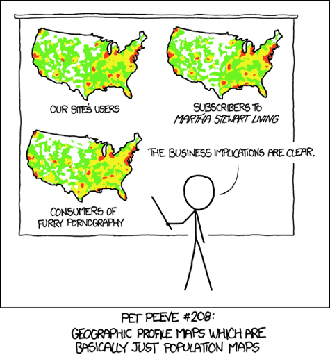
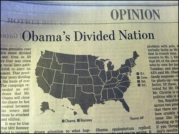
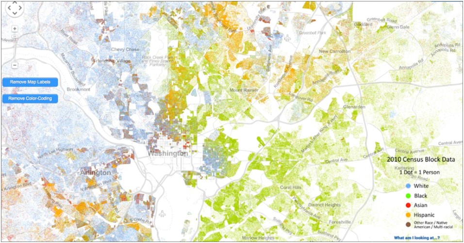
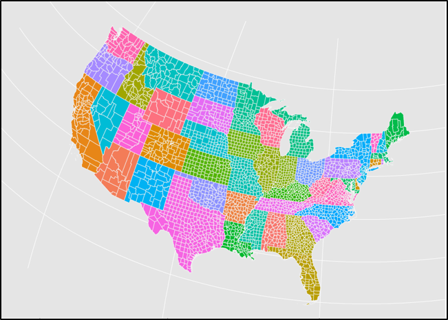
Intuitive
These two maps fall into traps. The left is a punchline, but the right is a typical mistake: using an ordered visual, one color hue along scaled saturation and values, to represent categorical values.
Red = Bad
Take advantage of R's color packages
Know your palettes
More can be more, but sometimes more can be less
Appropriate
These maps show how dramatically the analyst's choice of bucket values can impact the message of the map.
Why is a map more relevant than a bar/dist/scatter?
What are you trying to present to your audience?
Visually Appealing
One of the main reasons we use map graphics, even when a bar graph really would show the same information, is that it is visually compelling. We attach significance to the image as more "real" and we can double down on this irrational inflation of importance by making the graphic attractive.
Mapping in R
Why R?
We'll cover:
Why R is a preferred platform for generating map graphics
The single line of demo code to produce your first map graphic
An overview of how we can source our maps in R as a raster image or as vector and a comparison of these types' respective qualities
Examples produced in R implementing a series of classic map graphic overlays (dot density, graduated scale, choropleth, and isopleth)
Why R?
Free
Community supported
Attractive, informative, and fully reproducible graphics
R is free, the packages on which this presentation relies are free, they are open source (meaning we can look at the code to confirm it does what we intend, as can the entire R community), and there is a large body of active R users online offering tutorials, advice, and troubleshooting help.
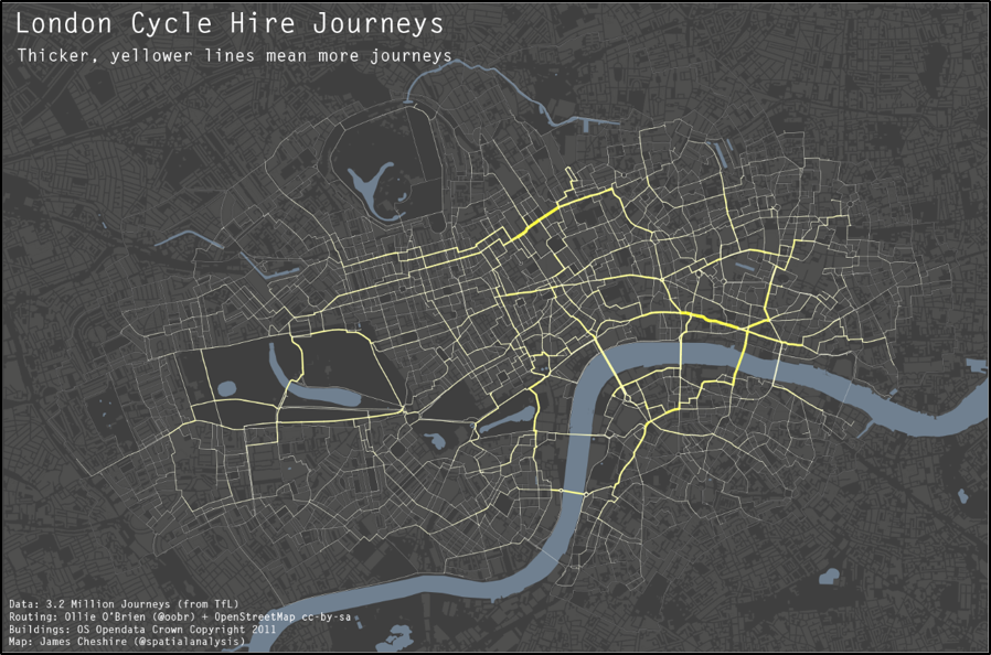
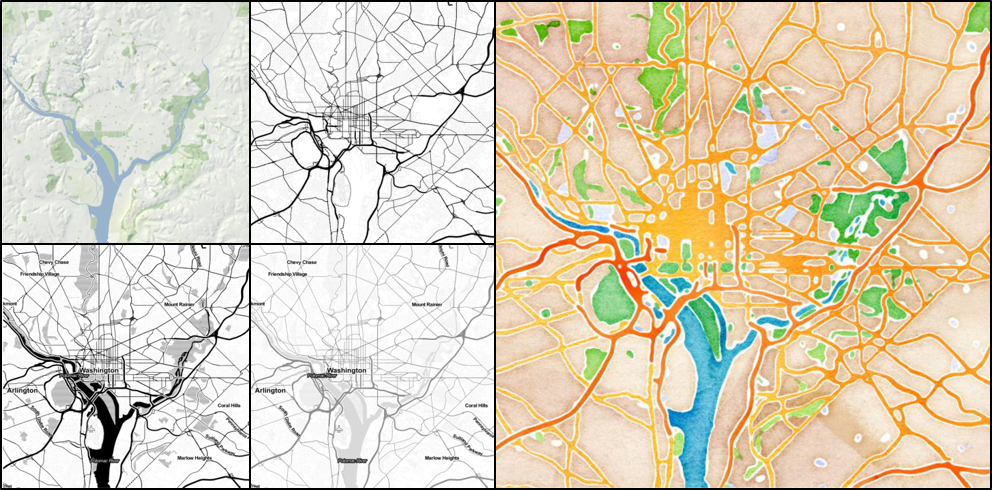
Why R.
This map was produced in R and is a gorgeous example of how far we can push reproducible map graphics.
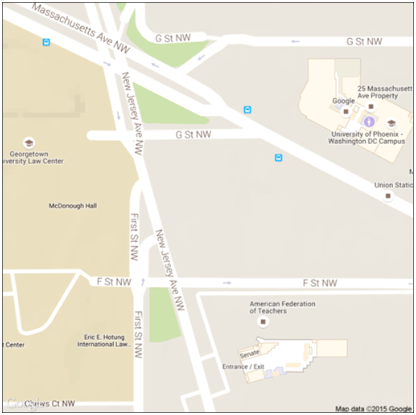
Your first map
qmap("601 New Jersey Ave NW, Washington, DC")
This is a map you can make by the end of today. We all start somewhere.
reference map (like we have here) or a topographic map (if we had pulled up a map showing hills, valleys, and bodies of water). What we care about as analysts are thematic maps which overlay information above the spatial and topographic features. You cannot call a map of London an "infographic," not even if it has streets, but you CAN if you visually encode those streets with traffic densities during rush hour.
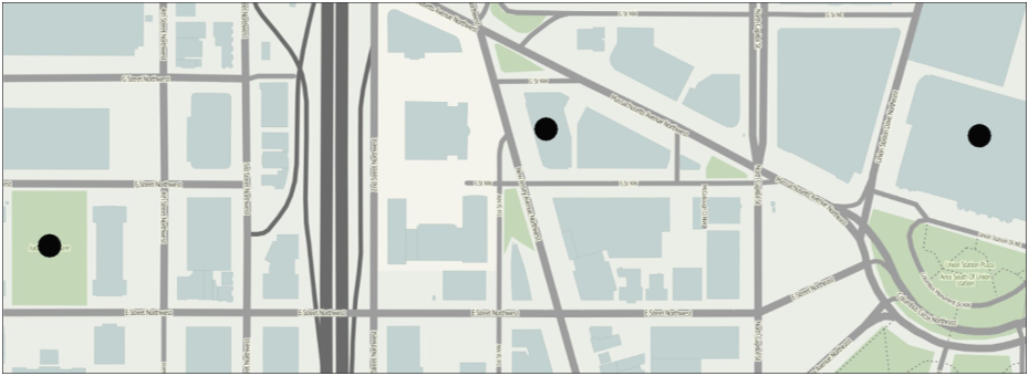
Your first map plot
eg <- data.frame(geocode(c("601 New Jersey Ave NW, Washington, DC",
                           "Union Station Metro, Washington, DC",
                           "Judiciary Square Metro, Washington, DC")))
qmplot(data = eg, x = lon, y = lat, zoom = 18, f = 1.1, size = I(3))
This is our first thematic map. It three locations: Summit Consulting and its flanking metro stations.
Rasters and Vectors
`qmap()` and `qplot()` are good starting points, especially for EDA, but they are unwieldy to use for customizing images. We're going to need to think about our MAP and our DATA separately.
Raster
A raster map is an image of a map
Appropriate for spatial point data
More attractive, more default options, less customizable
Vector
A vector map is composed of polygons
Appropriate for area-coded data
Customizable, flexible applications, less attractive for equivalent work
The best source of raster maps is the "ggmaps" package: it is easy to use, well documented, flexible, and created by two respected R developers (Wickham and Kahle).
EDA: "maps" and "choroplethr" packages. Easy-to-use datasets for common use cases like the globe, US states/counties, many more. Their weakness is how frequently their maps are updated (there is an apocryphal tale of the analyst mapping Europe and finding the Socialist Federal Republic of Yugoslavia proudly represented).
Production: it is straightforward to load shapefiles from trusted sources (e.g., US Census) into R. We will show an example of how this can be done.
Raster maps from `ggmap()`
ggmap(get_map("601 New Jersey Ave NW, Washington, DC",
              zoom = 12, source = "stamen", maptype = ...)
This is a small selection of the raster image types you can pull in using `ggmap()`. It accesses Google (limited API calls), Open Street Maps (limited API calls), Stamen Maps (no API limit and maptype calls appropriate to a variety of use cases).
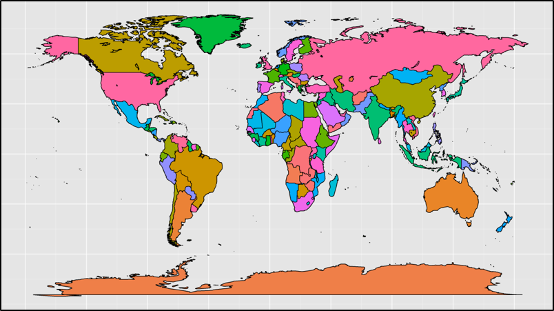
Vector maps from `maps`
map_data("world")
ggplot(world, aes(x = long, y = lat, group = group)) +
  geom_polygon(aes(fill = region), color = "black")
How did we make this map?
ElizabethAB/mapping_in_r .
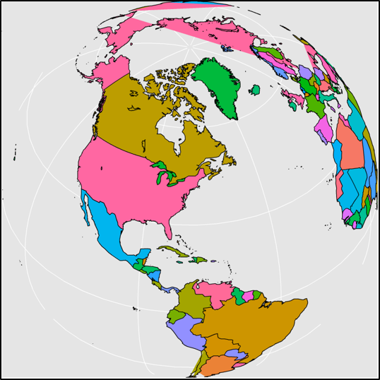
Vector maps from `maps`
map_data("world")
ggplot(world, aes(x = long, y = lat, group = group)) +
  geom_polygon(aes(fill = region), color = "black") +
  coord_map("ortho", orientation=c(41, -74, 0))
The value of vector maps is their customizability, easily accessed with the flexibility built into the "ggplot2" package.
The coord_map() call specifyies our preferred projection as orthographic and centers on New York City.
Projections are important to understanding maps, but are a complicated topic we won't cover thoroughly. In brief, map projections are mathematical transformations of a sphere to a flat plane representation and they necessarily trade off accuracy of angle, size, and relation. Different projection classes are better for accurately representing different latitudes (azimuthal for polar, cylindrical for equatorial, and conic for middle-latitude areas).
Vector maps from shapefiles
usa <- readOGR(dsn = "Inputs", "cb_2014_us_county_500k")
usa@data$id = rownames(usa@data)
usa.points = fortify(usa, region = "id")
county = join(usa.points, usa@data, by = "id")
Data source
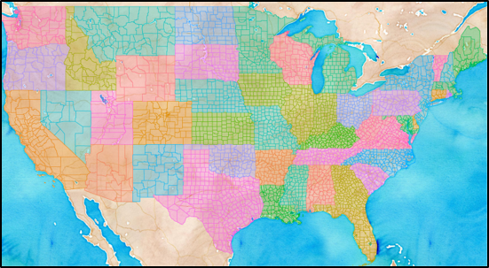
Mixing rasters and vectors
usa_raster <- get_map(bbox(county[,c("long", "lat")]),
                      maptype = "watercolor", zoom = 6)
ggmap(usa_raster, extent = "device",
      base_layer = ggplot(aes(x = long, y = lat, group = group),
                          data = county)) +
  geom_polygon(aes(fill = STATEFP, color = STATEFP), alpha = .3) +
  coord_map(projection = "mercator")
`county` is a dataframe containing the trace information for US counties. We source a watercolor type map (because it's pretty) using the bounding box of the `county` dataframe.
Graphing Data On Maps
Pulling in a map is an important step, but it won't mean much to us if we can't effectively overlay our data on it.
The following slides are examples of four basic graphic map types:
Dot density
Graduated symbol
Choropleth
Isopleth
The data used is the public HUD insured multifamily properties dataset and the US Census Quickfacts dataset .
In the following slides, we will review example cases of four classic map graphic types:
Dot density and graduated symbol maps are glorified scatter plots, but the superimposition of the information over a map allows us to draw inferences apparent only with the added spatial dimension.
Choropleth maps show concentrations or locations of statistical qualities broken down by administrative unit (you've probably seen colored voting pattern maps).
Isopleth maps represent abstract three dimensional surfaces to depict continuous phenomena (that is to say, an isopleth map can show you where in a city are concentrated the most positive Yelp reviews, or the most hipster Yelp reviews)
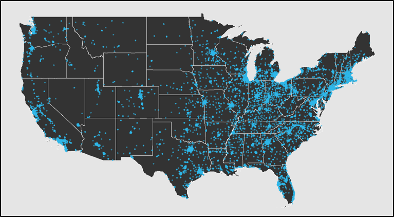
Dot density
ggplot(aes(x = long, y = lat), data = states) +
  geom_polygon(aes(group = group), color = "grey95") +
  geom_point(aes(x = LON, y = LAT), color = "#2db6e8", alpha = .6,
             data = insured) +
  coord_map()
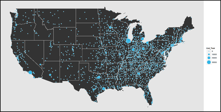
Graduated symbol
ggplot(aes(x = long, y = lat), data = states) +
  geom_polygon(aes(group = group), color = "grey95") +
  geom_point(aes(x = LON, y = LAT, size = Unit_Total), color = "grey85",
             data = cnty_count, shape = 21, fill = "#2db6e8") +
  coord_map()
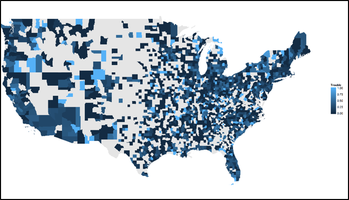
Choropleth
ggplot(aes(x = long, y = lat), data = county) +
  geom_polygon(aes(group = group, fill = Trouble)) +
  coord_map()
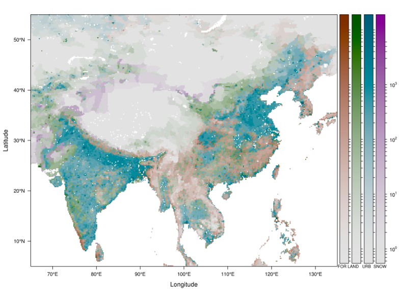
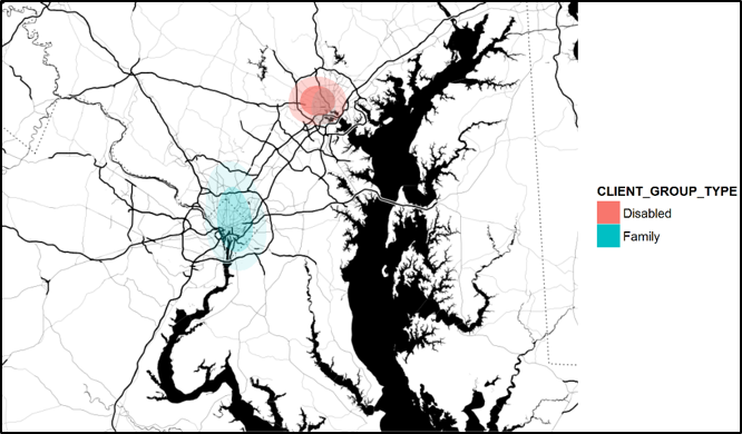
Isopleth
ggmap(dmv_map, base_layer =
        ggplot(aes(x = LON, y = LAT, fill = CLIENT_GROUP_TYPE),
               data = dmv_insured)) +
  stat_density2d(aes(alpha = ..level..), bins = 3, geom = "polygon")
Troubleshooting
An example: JPS's problem
JPS's Problem
Client presentation using geographic data
Want to highlight relative performance across states
Other mapping methods required proprietary software (SAS, ArcGIS), had limited customization (Excel), or required learning an entirely new open-source software on a short timeline (QGIS)
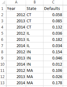
JPS's Problem
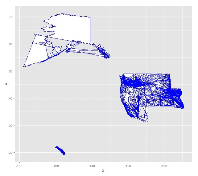
What the data look like:
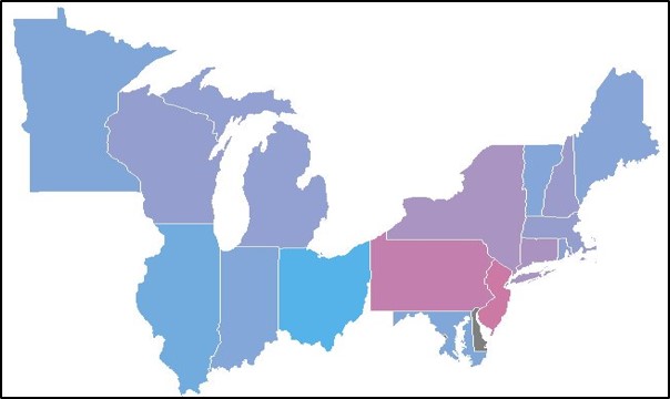
How we want the data to look:
How the data looked after plotting
Our first question is, what is the problem? As with all coding problems, defining the source of the issue is key to trying to solve it.
Troubleshooting
Typical sources of map graphic errors:
Graphic generator methods (e.g., `ggmap()` not recognizing variables provided by the base layer)
Data organization errors (e.g., ordering of vector points)
Projection mismatching (e.g., vector in WGS84 and data points in NAT83)
Clipping, Ordering, Color